

After introducing graphs and shortest path techniques like Dijkstra’s and Bellman-Ford’s algorithms, this article will introduce the following method: A* Search Algorithm.
The original article is available on Medium, and the Thai version of this article is available here.
Table of Contents
A* Search Algorithm
A* Search Algorithm [1] is a basis of Artificial Intelligence for finding an appropriate path between the start and the destination in a graph. This technique is suitable for a directed unweighted graph with non-negative edge weights.
This technique is similar to Dijkstra’s Algorithm. However, there is a little difference.
A* Search Algorithm uses an evaluation function [2]:
f(x) = g(x) + h(x)where
- g(x) is the actual cost of the node (or the distance to get to the node in the graph from a starting point)
- h(x) is the heuristic cost to reach a goal (or the estimation of the distance to get to the finish line from a node)
- and f(x) is a priority that combines between g(x) and h(x). f(x) considers whether that node is suitable for passing.
Process
A* search algorithm finds the appropriate path to traverse between the start (S) and the destination (G) by using the lowest cost. This technique requires two arrays:
- Open list or priority queue is an array that stores nodes with the lowest estimated cost (from f(x)) and waits for evaluation.
- Closed list is an array that stores evaluated nodes.
After defining an array, we use the open list to store the node with the lowest cost at the top and the highest cost at the bottom. This data structure is similar to a Min-Heap tree.
We summarize the process below.
Initialization
- Initialize the open and the closed lists.
- The open list initially contains only the start node as the root, while the closed list is empty.
- Set the cost of reaching the start node (or g(x)) to zero, get the heuristic cost (or h(x)), and calculate the actual cost (or f(x)).
The Loop
- Remove the root and place the node on the closed list.
- Search the neighbor nodes and loop inside to calculate the cost (or f(x)) to get the lowest one, which is a promising candidate for exploration.
- The node with the lowest cost is inserted into the open list and arranged to conform to the Min-Heap tree.
- Repeat the process until reaching the destination (G).
Use cases
Various tasks use an A* Search Algorithm: Robotics, Video Games, Route Planning, Logistics, and Artificial Intelligence [3].
- Robotics: A* algorithm assists the robot in navigating obstacles and finding an alternative path.
- Video Games: This algorithm plans NPCs (or Non-Player Characters) to navigate inside the game smartly.
- Route Planning: This technique provides the shortest path.
- Logistics: This task uses this technique to plan vehicle routes and schedules.
- Artificial Intelligence: This technique is utilized for natural language processing and machine learning to optimize decision-making processes.
Computational Complexity
Time Complexity equals O(b^d), where b is a branching factor that finds the average line in each node, and d is the number of nodes on the result path.
Space Complexity equals O(b^d).
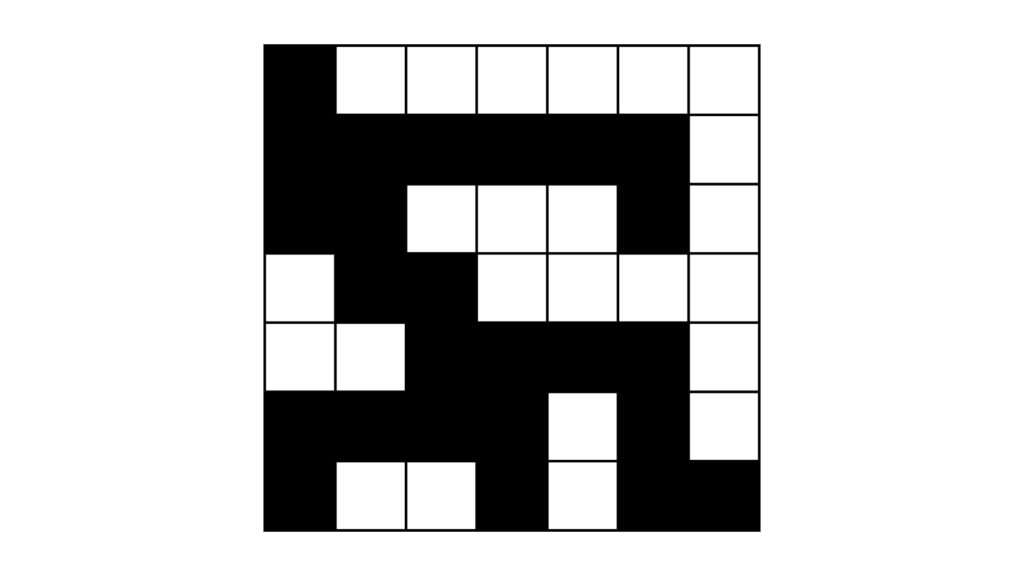
Traverse a maze
We want to travel in the maze shown in the picture below, with a defined starting point and a destination. Then, we want to use the computer to find the most appropriate path.

We can apply the A* search algorithm with the following processes.
Initialization
First, we create the maze variable as a class that contains
- walkability (1 = walkable, 0 = non-walkable)
- x and y coordinates
- parent coordinates
- heuristic costs (h(x))
- actual costs (g(x))
- and priorities (f(x)).
Then, we initialize the open and the closed set. The open set initially contains only the start node (at x = 0 and y = 0) as the root, while the closed set is empty.
After that, we set the costs (g(x), h(x), and f(x)) to zero.
The Loop
First, we remove the root and place the node in the closed list.
Second, we search the neighbor nodes from eight directions (Up, Down, Left, Right, Up-Left, Up-Right, Down-Left, and Down-Right). We consider three points.
- Consider whether the neighbor nodes are walkable (or walkability = 0).
- Check whether those nodes are in the closed list.
- Calculate f(x) to find the lowest cost by h(x) = current h(x) + 1, g(x) = Euclidian distance* from the current to the neighbor node, and f(x) = h(x) + g(x).
*Euclidian Distance [3] is the most common distance measure to find the length of a segment connecting two points.


Third, we insert the nodes with the lowest cost into the open list and arrange the list to conform to the Min-Heap Tree.
Fourth, loop the process from the first to the third until reaching the maze destination.
The Code
First, we import the essential libraries.
import heapq, copy, mathNext, we define a maze and a related class using the code below.
class Cell:
    def __init__(self, x, y, walkable):
        self.walkable = walkable      # Walkability
        self.x = x                    # X coordinate
        self.y = y                    # Y coordinate
        self.parent = [None, None]    # Parent coordinate
        self.h = float('inf')         # h(x)
        self.g = float('inf')         # g(x)
        self.f = float('inf')         # f(x)

maze = [
        ['1', '0', '0', '0', '0', '0', '0'],
        ['1', '1', '1', '1', '1', '1', '0'],
        ['1', '1', '0', '0', '0', '1', '0'],
        ['0', '1', '1', '0', '0', '0', '0'],
        ['0', '0', '1', '1', '1', '1', '0'],
        ['1', '1', '1', '1', '0', '1', '0'],
        ['1', '0', '0', '1', '0', '1', 'F'],
]

size_y = len(maze)
size_x = len(maze[0])
Third, we write a function to traverse a maze using an A* search algorithm, like the code below.
def isvalid(x, y, size_x, size_y):
    return x >= 0 and x < size_x and y >= 0 and y < size_y

# Calculate_h by Euclidian Distance
def calculate_h(source_x, source_y, dest_x, dest_y):
    return math.sqrt((source_x - dest_x) ** 2 +
                     (source_y - dest_y) ** 2)

def maze_astar(maze_orig, source_x = 0, source_y = 0,
               dest_x = 8, dest_y = 8, size_x = 4, size_y = 4):
    if source_y == dest_y and source_x == dest_x:
        print("This is a destination.")
        return [[source_x, source_y]]

    # Create Maze, Open and Closed List
    maze = [[Cell(j, i, maze_orig[i][j]) for j in range(size_x)] for i in range(size_y)]
    open = []
    heapq.heappush(open, (0.0, source_x, source_y))
    close = [[False for j in range(size_x)] for i in range(size_y)]

    # Direction
    direction = [
        ('U', 0, -1),
        ('D', 0, 1),
        ('F', 1, 0),
        ('B', -1, 0),
        ('UF', 1, -1),
        ('UB', -1, -1),
        ('DF', 1, 1),
        ('DB', -1, 1)
    ]

    # Initial
    maze[source_y][source_x].parent = None
    maze[source_y][source_x].f = 0
    maze[source_y][source_x].g = 0
    maze[source_y][source_x].h = 0

    found_dest = False

    while len(open) > 0:
        q = heapq.heappop(open)
        source_x, source_y = q[1:]
        close[source_y][source_x] = True

        # Check if we found the destination.
        if source_y == dest_y and source_x == dest_x:
            print("We found the destination")
            found_dest = True

            # Trace back
            dest_vertex = [source_x, source_y]
            path = []
            while True:
                path.append(dest_vertex)
                dest_vertex = maze[dest_vertex[1]][dest_vertex[0]].parent
                if dest_vertex is None:
                    break

            path.reverse()
            return path

        # Find Direction
        for name, add_x, add_y in direction:
            # New Coordinates
            neighbor_x, neighbor_y = source_x + add_x, source_y + add_y

            # Is not valid continue
            if not isvalid(neighbor_x, neighbor_y, size_x, size_y) or \
               maze[neighbor_y][neighbor_x].walkable == '0' or \
               close[neighbor_y][neighbor_x]:
               continue

            new_g = maze[source_y][source_x].g + 1
            new_h = calculate_h(source_x, source_y, neighbor_x, neighbor_y)
            new_f = new_h + new_g
            if maze[neighbor_y][neighbor_x].f == float('inf') or \
               new_f < maze[neighbor_y][neighbor_x].f:
                maze[neighbor_y][neighbor_x].parent = [source_x, source_y]
                maze[neighbor_y][neighbor_x].f = new_f
                maze[neighbor_y][neighbor_x].g = new_h
                maze[neighbor_y][neighbor_x].h = new_g

                heapq.heappush(open, (new_f, neighbor_x, neighbor_y))

    if not found_dest:
        print("We cannot found dest.")
        return []

    return None
Final, we write the code to let the algorithm traverse a maze.
output = maze_astar(maze, 0, 0,
size_x - 1, size_y - 1,
size_x, size_y)
visualize_maze = copy.deepcopy(maze)
for x, y in output:
visualize_maze[y][x] = 'X'
for i in range(size_y):
for j in range(size_x):
print(visualize_maze[i][j], end = '')
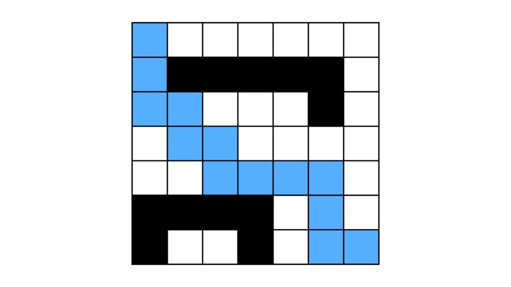
print('')The result is provided in the picture below. The blue one is an appropriate path provided by the algorithm from the start to the destination.
Summary
A* Search algorithm is a graph traversal technique for finding the most appropriate path between the start and the destination in a graph. This technique is popular in various tasks, such as Robotics, Video Games, Route Planning, Logistics, and Artificial Intelligence.
In this article, we apply the algorithm for route planning to traverse a maze to get the most appropriate path to walk from the start to the destination.
If you found this content useful, press Clap, and share it to various social media platforms. Moreover, readers can follow me on Linkedin or X (or Twitter).

